Getting started

FASTAR offers a large number of ways to interact with the synthesis of evolutionary stellar population models. This notebook offers a quick guide through the most basic functionalities

from matplotlib import pyplot as plt

Generating a standard SSP model (for spectroscopy)

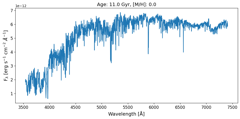
If you are interested in analyzing of spectrocopic data, these are most likely your models.

# Let's load the SSP synthesizer and an IMF
from fastar import IntegratedSSPSynthesizer
from fastar.imf import kroupa

# Now we can initialize the synthesizer
ssp = IntegratedSSPSynthesizer(imf_function=kroupa)

# Now you can generate SSP models for any age and metallicity
age = 11.0
met = 0.0

# Synthesize SSP
spec = ssp.synthesize(age=age, met=met)
wavelength = ssp.wave

# Let's see how it looks
figsize = (10, 5)
fig, ax = plt.subplots(figsize=(10, 5))
ax.plot(wavelength, spec)
ax.set_xlabel('Wavelength [Å]', fontsize=14)
ax.set_ylabel('F$_\lambda$ [erg s$^{-1}$ cm$^{-2}$ $\AA^{-1}$]', fontsize=14)
ax.set_title(f'Age: {age} Gyr, [M/H]: {met}', fontsize=14)
ax.tick_params(labelsize=12)

fig.tight_layout()
plt.show()

<>:21: SyntaxWarning: invalid escape sequence '\l'
<>:21: SyntaxWarning: invalid escape sequence '\l'
/tmp/ipykernel_1331/602161341.py:21: SyntaxWarning: invalid escape sequence '\l'
  ax.set_ylabel('F$_\lambda$ [erg s$^{-1}$ cm$^{-2}$ $\AA^{-1}$]', fontsize=14)

Generating a standard SSP model (for photometric analysis)

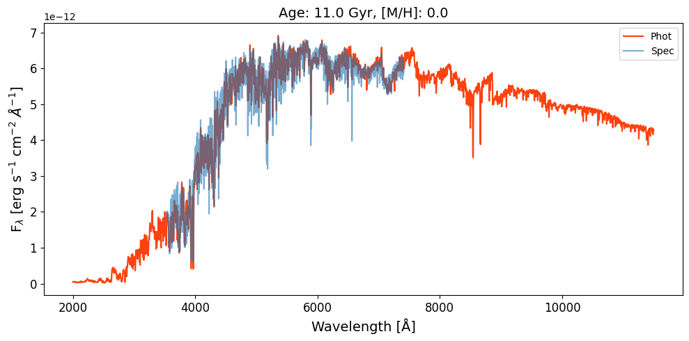
If you have photometric data beyond the spectroscopic coverage of FASTAR, don’t worry, you can use instead our photometric models. They have a coarse wavelength sampling (Δλ=4Å) but cover a wider wavelength range so you can convolve them with your favorite set of photometric filters

# The calling sequence is the same, but specifying that you want the photometric predictions while loading the synthesizer
ssp_phot = IntegratedSSPSynthesizer(model_label='phot', imf_function=kroupa)

# Using the same age and metallicity as before
age = 11.0
met = 0.0

# Synthesize SSP
sed = ssp_phot.synthesize(age=age, met=met)
wavelength_phot = ssp_phot.wave

# Let's see how it looks
figsize = (10, 5)
fig, ax = plt.subplots(figsize=(10, 5))
ax.plot(wavelength_phot, sed, color='xkcd:orangered', label='Phot')
ax.plot(wavelength, spec, alpha=0.6, label='Spec')
ax.legend()
ax.set_xlabel('Wavelength [Å]', fontsize=14)
ax.set_ylabel('F$_\lambda$ [erg s$^{-1}$ cm$^{-2}$ $\AA^{-1}$]', fontsize=14)
ax.set_title(f'Age: {age} Gyr, [M/H]: {met}', fontsize=14)
ax.tick_params(labelsize=12)

fig.tight_layout()
plt.show()

<>:19: SyntaxWarning: invalid escape sequence '\l'
<>:19: SyntaxWarning: invalid escape sequence '\l'
/tmp/ipykernel_1331/2323936794.py:19: SyntaxWarning: invalid escape sequence '\l'
  ax.set_ylabel('F$_\lambda$ [erg s$^{-1}$ cm$^{-2}$ $\AA^{-1}$]', fontsize=14)

Generating a semi-resolved SSP model

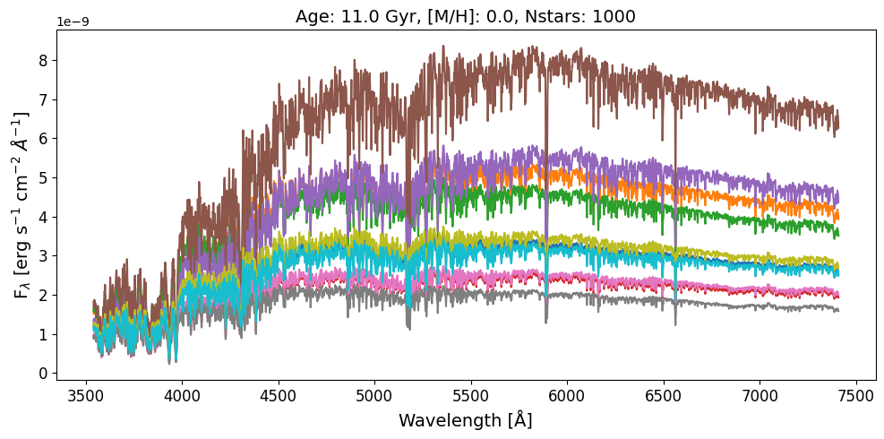
A unique feature of FASTAR is the possibility of generating SSP models for semi-resolved stellar populations, i.e., without assuming an infinite number of stars contributing to the spectrum. Synthesizing these models is also straight-forward, with only an additional free parameter determining the number of stars you want in your model.

# The synthesis is rather similar although we also need to import a JAX key generator for the IMF sampling
import jax
from fastar import SemiresolvedSSPSynthesizer

# Now we can load the semi-resolved synthesizer
semi = SemiresolvedSSPSynthesizer(imf_function=kroupa)

# Generate the key
key = jax.random.PRNGKey(0)

# And then simply synthesize a semi-resolved model
age = 11.0
met = 0.0
nstars = 1000

# Synthesize SSP
semi_model, semi_stellar_mass = semi.synthesize(
    age=age, met=met, num_stars=int(nstars), key=key
)

A single semi-resolved model doesn’t probably say may because they are stochastic and thus predictions are not unique even with the same age, metallicity, IMF and number of stars. Let’s do a bunch of them instead

# We first define the number of models and split the random key
nmodels = 10
keys = jax.random.split(key, nmodels)

figsize = (10, 5)
fig, ax = plt.subplots(figsize=(10, 5))

for i in range(nmodels):
    semi_model, _ = semi.synthesize(
        age=age, met=met, num_stars=int(nstars), key=keys[i]
    )
    plt.plot(wavelength, semi_model)
ax.set_xlabel('Wavelength [Å]', fontsize=14)
ax.set_ylabel('F$_\lambda$ [erg s$^{-1}$ cm$^{-2}$ $\AA^{-1}$]', fontsize=14)
ax.set_title(f'Age: {age} Gyr, [M/H]: {met}, Nstars: {nstars}', fontsize=14)
ax.tick_params(labelsize=12)

fig.tight_layout()
plt.show()

<>:14: SyntaxWarning: invalid escape sequence '\l'
<>:14: SyntaxWarning: invalid escape sequence '\l'
/tmp/ipykernel_1331/1355448506.py:14: SyntaxWarning: invalid escape sequence '\l'
  ax.set_ylabel('F$_\lambda$ [erg s$^{-1}$ cm$^{-2}$ $\AA^{-1}$]', fontsize=14)

Optimal ages and metallicities

If you are not interested in the continuity of the FASTAR models you may want to have a fixed array of ages and metallicities as standard SSP models. Replicating the most common approach, you can use the age and metallicity grid of the underlying isochrones. In FASTAR they are easily accessible

age_basti = ssp.ages / 1000.0  # Myr -> Gyr
met_basti = ssp.mets

However, FASTAR can take a step forward and use its differentiable nature to provide an optimal age and metallicity sampling. This sampling in age and metallicity ensures a constant variation in the spectra of consecutive bins. If you need a grid of ages and metallicities, these are likely the values where you want to evaluate the models

age_optimal = ssp.iso_ages  # By default these are already in Gyr
met_optimal = ssp.iso_mets