IMF variations in FASTAR

To synthesize a new SSP model, the first step is always to specify the IMF parametrization while loading the synthesizer.

import numpy as np
from matplotlib import pyplot as plt
from matplotlib.ticker import ScalarFormatter

from fastar import IntegratedSSPSynthesizer
from fastar import imf

# Load the SSP synthesizer with a Salpeter-like IMF (single power law)
ssp = IntegratedSSPSynthesizer(imf_function=imf.single_power_law)

# Generate an SSP model (10 Gyr, solar metallicity for example)
spec = ssp.synthesize(age=10, met=0)

Pre-defined functional forms

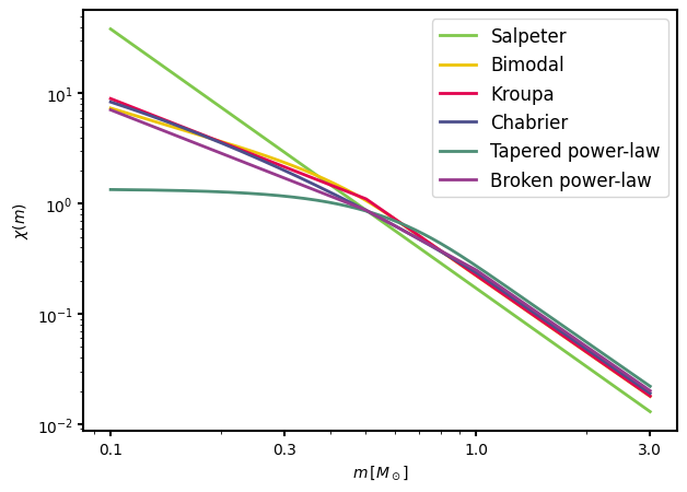
FASTAR comes with 6 pre-defined funtional forms. Let’s have a look at them

# To plot the different IMF, we first define a range of stellar masses
mass = np.linspace(0.1, 3, 1000)

# Then we can load all the different IMFs with their default parameters
bimodal = imf.bimodal(mass, params={})
salpeter = imf.single_power_law(mass, params={})
flexi = imf.flexi(mass, params={})
broken = imf.broken_power_law(mass, params={})
kroupa = imf.kroupa(mass, params={})
chabrier = imf.chabrier(mass, params={})

# Now we can see how they look
fig, ax = plt.subplots(figsize=(7, 5))

colors = {
    'Bimodal': '#edc407ff',
    'Salpeter': '#80c84cff',
    'Flexi': '#4d8e76ff',
    'Broken': '#973a8dff',
    'Kroupa': '#e2044fff',
    'Chabrier': '#4c4e8bff',
}

ax.plot(mass, salpeter, linewidth=2, label='Salpeter', color=colors['Salpeter'])
ax.plot(mass, bimodal, linewidth=2, label='Bimodal', color=colors['Bimodal'])
ax.plot(mass, kroupa, linewidth=2, label='Kroupa', color=colors['Kroupa'])
ax.plot(mass, chabrier, linewidth=2, label='Chabrier', color=colors['Chabrier'])
ax.plot(mass, flexi, linewidth=2, label='Tapered power-law', color=colors['Flexi'])
ax.plot(mass, broken, linewidth=2, label='Broken power-law', color=colors['Broken'])

leg = ax.legend(fontsize=12)
for line in leg.get_lines():
    line.set_linewidth(2)

ax.set_xscale('log')
ax.set_yscale('log')
ax.set_xlabel(r'$m \, [M_\odot]$')
ax.set_ylabel(r'$\chi(m)$')

ax.set_xticks([0.1, 0.3, 1, 3])
ax.get_xaxis().set_major_formatter(ScalarFormatter())

ax.tick_params(width=1.5, axis='both')
for spine in ax.spines.values():
    spine.set_linewidth(1.5)

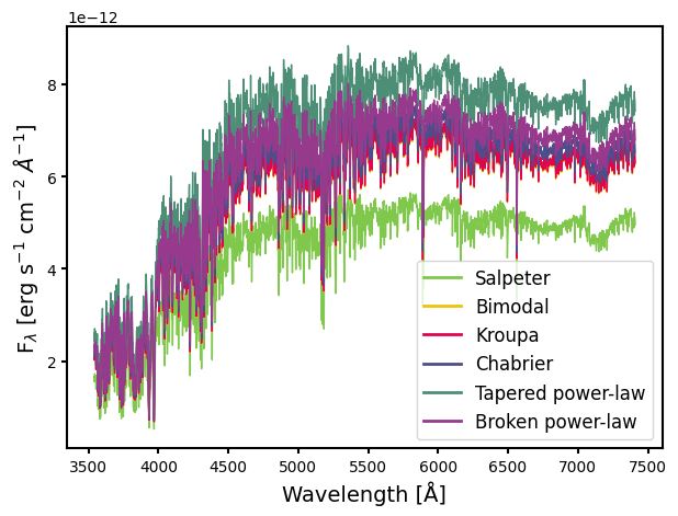
Now that we know how they look, let’s generate SSP models with the same age and metallicity but different IMFs

# Create six different synthesizers
ssp_single_power_law = IntegratedSSPSynthesizer(imf_function=imf.single_power_law)
ssp_bimodal = IntegratedSSPSynthesizer(imf_function=imf.bimodal)
ssp_flexi = IntegratedSSPSynthesizer(imf_function=imf.flexi)
ssp_broken_power_law = IntegratedSSPSynthesizer(imf_function=imf.broken_power_law)
ssp_kroupa = IntegratedSSPSynthesizer(imf_function=imf.kroupa)
ssp_chabrier = IntegratedSSPSynthesizer(imf_function=imf.chabrier)

# Synthesize the six SSPs
spec_single_power_law = ssp_single_power_law.synthesize(age=10, met=0)
spec_bimodal = ssp_bimodal.synthesize(age=10, met=0)
spec_broken_power_law = ssp_broken_power_law.synthesize(age=10, met=0)
spec_flexi = ssp_flexi.synthesize(age=10, met=0)
spec_kroupa = ssp_kroupa.synthesize(age=10, met=0)
spec_chabrier = ssp_chabrier.synthesize(age=10, met=0)

wave = ssp_chabrier.wave

# Finally plotting all the spectra
fig, ax = plt.subplots(figsize=(7, 5))

colors = {
    'Bimodal': '#edc407ff',
    'Salpeter': '#80c84cff',
    'Flexi': '#4d8e76ff',
    'Broken': '#973a8dff',
    'Kroupa': '#e2044fff',
    'Chabrier': '#4c4e8bff',
}

ax.plot(
    wave, spec_single_power_law, linewidth=1, label='Salpeter', color=colors['Salpeter']
)
ax.plot(wave, spec_bimodal, linewidth=1, label='Bimodal', color=colors['Bimodal'])
ax.plot(wave, spec_kroupa, linewidth=1, label='Kroupa', color=colors['Kroupa'])
ax.plot(wave, spec_chabrier, linewidth=1, label='Chabrier', color=colors['Chabrier'])
ax.plot(wave, spec_flexi, linewidth=1, label='Tapered power-law', color=colors['Flexi'])
ax.plot(
    wave,
    spec_broken_power_law,
    linewidth=1,
    label='Broken power-law',
    color=colors['Broken'],
)

leg = ax.legend(fontsize=12)
for line in leg.get_lines():
    line.set_linewidth(2)


ax.set_xlabel('Wavelength [Å]', fontsize=14)
ax.set_ylabel('F$_\lambda$ [erg s$^{-1}$ cm$^{-2}$ $\AA^{-1}$]', fontsize=14)

ax.tick_params(width=1.5, axis='both')
for spine in ax.spines.values():
    spine.set_linewidth(1.5)

<>:52: SyntaxWarning: invalid escape sequence '\l'
<>:52: SyntaxWarning: invalid escape sequence '\l'
/tmp/ipykernel_1639/3108150441.py:52: SyntaxWarning: invalid escape sequence '\l'
  ax.set_ylabel('F$_\lambda$ [erg s$^{-1}$ cm$^{-2}$ $\AA^{-1}$]', fontsize=14)

Changing the IMF parameters

Each of the available functional forms has a set of parameters determining its actual shape. FASTAR has been coded with the idea of giving the user the freedom to generate SSP models for arbitrary combination of parameters.

Important note

Changing the IMF mass limits (m_min, m_max) can significantly impact quantities such as mass-to-light ratios. However, it can also quickly lead to non-physical or unreliable model predictions.

With great power comes great responsibility.

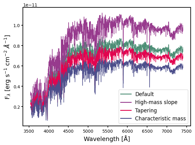
The free parameters of each IMF are described in the documentation and in the FASTAR papers. The synthesis flexibility can be illustrated, for example, with the tapered power-law IMF of de Marchi, Paresce & Portegies Zwart (2005). Changes in the IMF parameters are passed through a dictionary.

# Let's use as reference the default values
spec_ref = ssp_flexi.synthesize(age=10, met=0)

# Change in the high-mass end slope (default alpha = 2.3)
spec_var1 = ssp_flexi.synthesize(age=10, met=0, imf_params={'alpha': 3})

# Sharpness of the exponential taper (default beta = 2.3)
spec_var2 = ssp_flexi.synthesize(age=10, met=0, imf_params={'beta': 1.5})

# Varying the characteristic mass (default m_peak = 0.5)
spec_var3 = ssp_flexi.synthesize(age=10, met=0, imf_params={'m_peak': 0.2})

# Plotting all the spectra
fig, ax = plt.subplots(figsize=(7, 5))

colors = {
    'Ref': '#4d8e76ff',
    'Var1': '#973a8dff',
    'Var2': '#e2044fff',
    'Var3': '#4c4e8bff',
}

ax.plot(wave, spec_ref, linewidth=1, label='Default', color=colors['Ref'])
ax.plot(wave, spec_var1, linewidth=1, label='High-mass slope', color=colors['Var1'])
ax.plot(wave, spec_var2, linewidth=1, label='Tapering', color=colors['Var2'])
ax.plot(wave, spec_var3, linewidth=1, label='Characteristic mass', color=colors['Var3'])

leg = ax.legend(fontsize=12)
for line in leg.get_lines():
    line.set_linewidth(2)


ax.set_xlabel('Wavelength [Å]', fontsize=14)
ax.set_ylabel('F$_\lambda$ [erg s$^{-1}$ cm$^{-2}$ $\AA^{-1}$]', fontsize=14)

ax.tick_params(width=1.5, axis='both')
for spine in ax.spines.values():
    spine.set_linewidth(1.5)

<>:34: SyntaxWarning: invalid escape sequence '\l'
<>:34: SyntaxWarning: invalid escape sequence '\l'
/tmp/ipykernel_1639/1539093115.py:34: SyntaxWarning: invalid escape sequence '\l'
  ax.set_ylabel('F$_\lambda$ [erg s$^{-1}$ cm$^{-2}$ $\AA^{-1}$]', fontsize=14)

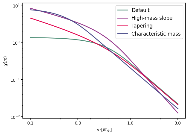
For consistency, it is also possible to have a look at the changes in the shape of the IMF

flexi_ref = imf.flexi(mass, params={})
flexi_var1 = imf.flexi(mass, params={'alpha': 3})
flexi_var2 = imf.flexi(mass, params={'beta': 1.5})
flexi_var3 = imf.flexi(mass, params={'m_peak': 0.2})

fig, ax = plt.subplots(figsize=(7, 5))

ax.plot(mass, flexi_ref, linewidth=2, label='Default', color=colors['Ref'])
ax.plot(mass, flexi_var1, linewidth=2, label='High-mass slope', color=colors['Var1'])
ax.plot(mass, flexi_var2, linewidth=2, label='Tapering', color=colors['Var2'])
ax.plot(
    mass, flexi_var3, linewidth=2, label='Characteristic mass', color=colors['Var3']
)

leg = ax.legend(fontsize=12)
for line in leg.get_lines():
    line.set_linewidth(2)

ax.set_xscale('log')
ax.set_yscale('log')
ax.set_xlabel(r'$m \, [M_\odot]$')
ax.set_ylabel(r'$\chi(m)$')

ax.set_xticks([0.1, 0.3, 1, 3])
ax.get_xaxis().set_major_formatter(ScalarFormatter())

ax.tick_params(width=1.5, axis='both')
for spine in ax.spines.values():
    spine.set_linewidth(1.5)